In actuarial science, data analysis is a fundamental part of the job, whether you’re working on reserving models, pricing, or risk management. One of the most essential early steps in any data project is exploratory data analysis (EDA) — and that starts with understanding the distribution of your variables. While summary statistics are useful, they often hide important nuances. That’s where visualizations come in.
A well-constructed plot can quickly reveal skewness, multimodality, and outliers — all of which might impact your models. For example, before using a variable in a predictive model, you’d want to know whether it’s heavily skewed, has a long tail, or contains extreme values that could distort your results.
To help with this, let’s look at a simple yet powerful function in Python that combines two key plots: a boxplot and a histogram. Together, they provide both a compact summary and a detailed view of a variable’s distribution — ideal for any univariate analysis.
Here is the function, explained step by step:
import matplotlib.pyplot as plt
import seaborn as sns
set.sns() # default aesthetics (makes plots look better with minimal effort!)
def hist_box(data, var):
"""
Plot a boxplot and histogram (with KDE) for a given variable in a dataset.
Parameters:
data (pd.DataFrame): The input DataFrame containing the variable to plot.
var (str): The name of the column/variable to visualize.
"""
# Create a figure with two subplots: one for the boxplot, one for the histogram
fig, (ax_box, ax_hist) = plt.subplots(
2, # 2 rows of plots
sharex=True, # Share the same x-axis
gridspec_kw={'height_ratios': (0.15, 0.85)}, # Relative heights of the plots
figsize=(12, 6) # Size of the entire figure
)
# Set a main title for the figure
fig.suptitle(f'Distribution of {var}', fontsize=14)
# Remove default figure margins for better use of space
plt.margins(0)
# Draw the boxplot (compact summary of distribution)
sns.boxplot(data=data, x=var, ax=ax_box, showmeans=True)
ax_box.set(xlabel='') # Remove x-axis label from the boxplot for clarity
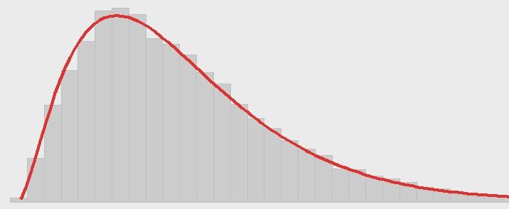
# Draw the histogram with KDE (detailed distribution)
sns.histplot(data=data, x=var, kde=True, ax=ax_hist)
# Display the combined plot
plt.tight_layout(rect=[0, 0, 1, 0.96]) # Adjust layout to fit the suptitle
plt.show()Once you have defined this function, you can use it with any numerical variable in a pandas DataFrame. For instance, if you’re working with policyholder data and want to explore the distribution of claim amounts, you’d simply call:
hist_box(df, 'claim_amount')
This gives you an instant view of both the central tendency and the shape of the distribution. The boxplot makes it easy to detect outliers, while the histogram and KDE curve help you understand whether the data is symmetric, skewed, or possibly multimodal.
Functions like this are especially helpful when you’re analyzing multiple variables. You could easily put this in a loop and generate dozens of distribution plots to assess data quality before modeling.
As you grow in your actuarial career, mastering basic EDA techniques like this one will help you uncover valuable insights and communicate findings more effectively — whether to peers, clients, or regulators. Plus, getting comfortable with Python early on gives you a head start in today’s increasingly data-driven profession.